An Exploration of Parallel Computing

What is Parallel Computing?

Parallel computing is a computational technique where multiple tasks or operations are executed simultaneously, leveraging multiple processors, cores, and/or computers over a network to solve problems more efficiently than traditional sequential processing. By dividing a problem into smaller, manageable parts that can be processed concurrently, parallel computing significantly speeds up computations. In this blog, I will be sharing the results of my informal exploration into the world of parallel computing.

How Did I Get Here?

Like many of the endeavors I have taken in my computer science journey, it always start out as a simple question before I inevitably descend into an endless rabbit hole. In this particular case, it began as a question on a Saturday night several months ago on how to reduce a CPU bottleneck in a video game. Then, in a series of events, I ended up reading the spec sheets and documentation for my CPU and GPU, which is an AMD Zen 4 processor and a Radeon 7000 series graphics card, respectively.

The documentations described using SIMD (single instruction, multiple data) and SIMT (single instruction, multiple thread) instructions to parallelize computations. It’s a fairly easy concept to understand at a high level. However, I am a firm believer that I needs to try something for myself to truly understand. This is where my exploration of SIMD/SIMT instructions, GPU programming, and CPU multi-threading began.

Exploration Begins!

First, I need to define a set of control scenarios for my experiments. For the sake of demonstrating, I chose a highly parallel task of applying arithmetic operations to an array of numbers. Although many real world scenarios cannot be easily refactored to smaller parallel tasks, this example will suffice.

Experimental Data:

Traditional Single-Threaded Processing:

In a traditional computer program, a processor must access each element and perform the operation one-by-one in sequence. Although modern CPUs use techniques such as instruction pipelining and out-of-order execution to take advantage of some amount of instruction level parallelism, the overall execution is still sequential.

To demonstrate single-thread processing in action and to use this as a baseline comparison for my experiments, I’ve written a C++ program that simulate a workload on 1 billion single-precision floating point numbers by incrementing each element by one for a number of iterations.

// Single-threaded workload
void count_function(float* a, long int size, int iterations) {
  for (int j = 0; j < iterations; j++) {
    for (int i = 0; i < size; i++) {
      a[i] += 1;
    }
  }
}

I also made a modification to swap the inner and outer loop in an attempt to take advantage of cache locality. Although this produced no benefits in this test, this will become important in later explorations.

// Modified single-threaded workload
void count_function(float* a, long int size, int iterations) {
  for (int i = 0; i < size; i++) {
    for (int j = 0; j < iterations; j++) {
      a[i] += 1;
    }
  }
}

In both versions of the single-threaded test, it took about 15-16 seconds to complete 10 iterations. This will be the baseline of my comparison moving forward.

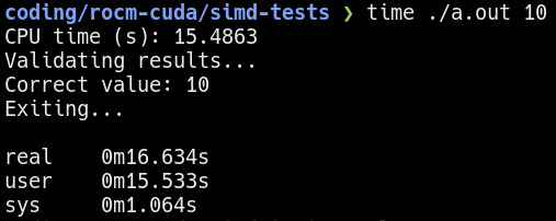Single-threaded benchmark using 10 iterations

It is important to verify the assembly instructions emitted by the compiler to ensure no fancy shortcuts are used to compute the simulated workload. For example, a compiler optimization might be to compute one element and then apply it to the other elements.

Multi-threaded Processing:

The logical continuation of this exploration is to rewrite the program to use multi-threading. By parallelizing the workload between multiple threads, the performance should speed-up by factors proportional to the number of threads. Note that the core workload functions defined above is unmodified. Only the main function is modified to launch multiple threads.

#define NUM 1000000000
int main() {
  /* ... */
  std::thread threads[THREADS];

  long int chunk_size = NUM / THREADS;
  for (int j = 0; j < THREADS; j++) {

    int chunk_start = chunk_size * j;
    threads[j] = std::thread(count_function, &a[chunk_start], chunk_size, iterations);
  }
  for (int j = 0; j < THREADS; j++) {
    threads[j].join();
  }
  /* ... */
}

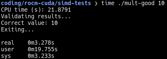Multi-threaded benchmark using 10 iterations

The CPU time measured is the sum of the processing time used by all threads. The real time give a more accurate estimate of the execution time. Moving forward, all comparisons will use the real time.

Using multi-threading on a 6 core 12 threads Zen 4 processor, it takes about 3 seconds to complete the same workload. If I were to keep the processing time constant (see below), the multi-threaded program is able to process about 7 times more!

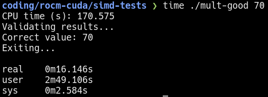Multi-threaded benchmark using 70 iterations

Please note that there are overhead associated with launching and joining threads. Also, Hyper-threading/SMT do not exactly double the performance. Therefore, the total speed-up is not 12 times faster.

SIMD Instructions:

Here is where the interesting part begins. On modern processors, there are special instructions programmers can use to “bundle up” data for the CPU to process all at once. These instructions are called SIMD (single instruction, multiple data) instructions.

A simplified overview of SIMD is that multiple numbers are placed in a wide SIMD register. The processor then can operate on the entire SIMD register in a single cycle¹.

Depending on processor architecture, the size of the SIMD register typically vary from 128 to 512 bits wide. Although the SIMD extensions such as AVX512 specifies 512-bit wide support, the underlying processor architecture do not necessarily implement a physical 512-bit wide register. In fact, a Zen 4 core implements what AMD calls a “double-pumping” strategy where a 512-bit wide SIMD instruction is broken into two 256-bit wide operations. A comparison between compiling with AVX2 (256-bits) and AVX512 (512-bits) seems to confirm this.

Writing or transforming a program to use SIMD instructions is easy. Assuming the processor actually supports SIMD instructions, all that needs to be done is pass the appropriate flags to the compiler. Modern compilers such as gcc/g++ or clang/clang++ can easily emit code for SIMD instructions.

On Linux, you can check if SIMD and other features are supported by reading the /proc/cpuinfo file.

Here, I recompiled the multi-threaded program using the -mavx512f option.

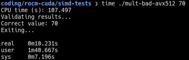Performance of running 70 iterations of the “bad” workload

Hmm…the results improved from before, but not by much. Why is that? Remember I mentioned there are two versions of the single-threaded workload? The result shown is using the unmodified workload, where the outer loop is the iterations and inner loop accesses the elements. As a refresher, here it is again:

// "Bad" workload
void count_function(float* a, long int size, int iterations) {
  for (int j = 0; j < iterations; j++) {
    for (int i = 0; i < size; i++) {
      a[i] += 1;
    }
  }
}

But why is this bad? My hypothesis is that the “bad” workload written in a way that destroys spacial cache locality. For each iteration, the inner loop is going through all X number of elements where X >> size of the data cache in the CPU. This means that the data cache is constantly flushed and reloaded from memory due to cache misses, which is slow.

The alternative workload shown below prevents this by operating on each element repeatedly before moving to the next. The CPU only needs to load the element once into cache and subsequent accesses/write-backs will have the value in cache. Additionally, modern processors load memory in chunks, so adjacent elements in the array will also get cache locality benefits.

// "Good" workload
void count_function(float* a, long int size, int iterations) {
  for (int i = 0; i < size; i++) {
    for (int j = 0; j < iterations; j++) {
      a[i] += 1;
    }
  }
}

Running the “good” version of the program yields a much better result. Keeping the execution time at about 15 seconds, I observe over 30x increase in performance compared to the single-threaded baseline. 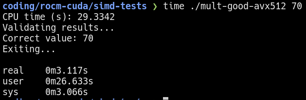Performance of running 70 iterations of the “good” workload 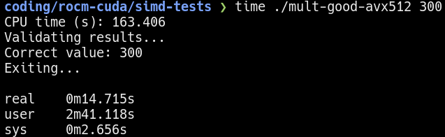Performance of running 300 iterations of the “good” workload

Verifying the Cache Locality Hypothesis:

On Linux, the perf utility can be used to measure performance metrics of a program. Using the command perf stat -d time <program>, I can measure some cache behaviors.

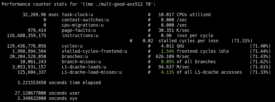Cache behavior of the “good” workload 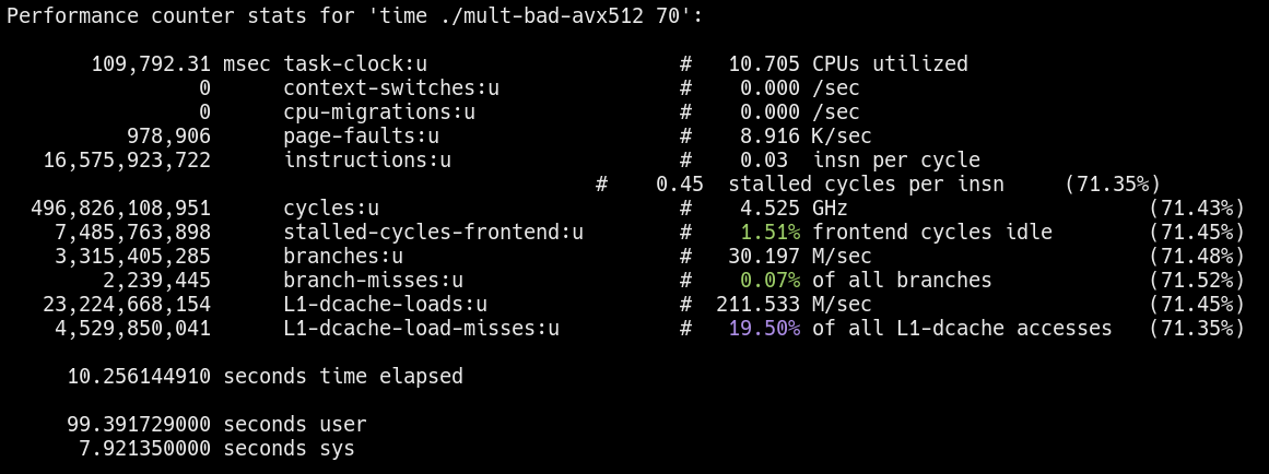Cache behavior of the “bad” workload

Notice the L1-dcache-load-misses for the “bad” workload is significantly higher as expected. More evidence is needed, but preliminary results seem to support my hypothesis.

According to some sources, the sampling used to measure cache performance can vary between CPU architectures.

GPU Acceleration/SIMT Instructions:

So far, I’ve only been using CPU parallel programming to get more performance, but the CPU is not known for doing this type of work. Instead, the GPU is highly efficient in parallel workloads. The reason why GPUs excel in parallel computations is because of SIMT (single instruction, multiple threads) instructions. Similar to SIMD instructions, the SIMT model also parallelizes program execution. However, SIMT operates across threads rather than on data. In both Nvidia and AMD GPUs, the execution threads are organized where a single instruction is executed across the collection² of threads (typically in groups of 32).

For more information, visit Nvidia’s CUDA and AMD’s ROCm documentation.

Below is a code snippet of the example workload written using Heterogeneous-computing Interface for Portability (HIP). HIP programs are compatible with both Nvidia and AMD GPUs.

#define NUM 1000000000

__global__ void count_kernel(float* a, long int size, int iterations) {
  long int tid = blockIdx.x * blockDim.x + threadIdx.x;

  // Check to make sure no out of bounds access
  if (tid < size) {
    for (int i = 0; i < iterations; i++) {
      a[tid] += 1;
    }
  }
}

int main() {
  /* ... */
  int block_size = 256;
  int grid_size = (NUM + block_size - 1) / block_size;

  hipStream_t stream;
  HIP_ASSERT(hipStreamCreate(&stream));
  count_kernel<<<grid_size, block_size, 0, stream>>>(d_a, NUM, iterations);
  /* ... */
}

The result for a 300 iteration run on the GPU is shown below: 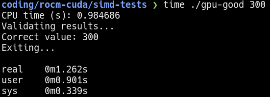300 iterations on the GPU

The GPU is so fast in computation that the data transfer time to and from the GPU is the dominating factor.

To get more accurate measurements, I increased the number of iterations to 10000 and 25000. 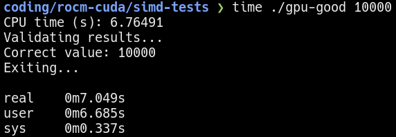10000 iterations on the GPU 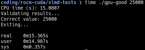25000 iterations on the GPU

Results:

Comparing the baseline single-threaded CPU performance with the GPU-accelerated performance reveals an impressive 2500x increase in performance. This substantial boost is attributed to the ability of GPUs to handle parallel tasks more efficiently than CPUs, especially when applications are optimized for GPU architectures. However, it’s important to note that achieving such a high performance improvement depends on several factors:

1. Application Suitability: The application must be well-suited for GPU acceleration, with minimal dependencies and a high degree of parallelism. This exploration arbitrarily chose a simple and highly parallel workload. It is overly optimistic to expect a similar boost in performance in real workloads.

2. Optimization Efforts: It is essential to have effective optimization of code to take full advantage of GPU features, such as shared memory and optimized data access patterns. A vram/cache bottleneck similar to the cache locality problem on the CPU can also be observed on the GPU. The vram experimental program/data is omitted because of it’s similarity to the CPU cache locality problem.

3. Measurement Contexts: The performance improvement was measured in terms of time taken to complete a task, indicating a significant reduction in computation time when using the GPU. However, it is important to note that GPUs can consume significantly more power. While still very impressive, the performance gained per power consumed is only about 800x (instead of 2500x) in this set of experiments.

While this exploration highlights the potential of GPU acceleration, it is important to interpret these results with appropriate context. For any workload, it must be viewed within the broader context of application suitability, optimization efforts, and measurement contexts.

Footnotes:

1. The instruction is not processed in a single clock cycle due to the pipelined nature of a processor. ↩︎

2. This collection of threads as known as a warp (Nvidia) or a wavefront (AMD). ↩︎